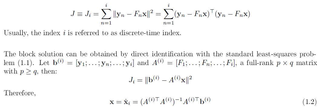
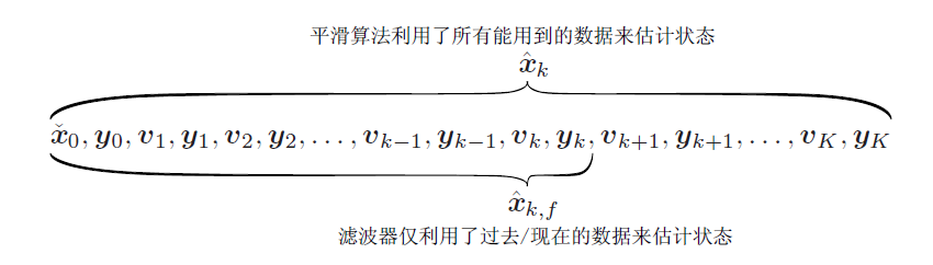
Estimation Machinery
K3 Linear-Gaussian Estimation - 2
上回小结
K3主要分析 线性高斯系统(LG)
首先将LG系统抽象为运动方程和观测方程
So 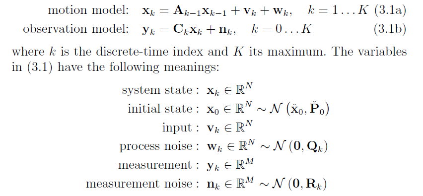
目的是求解: 系统状态 x, 即 $\hat{x}$ 后验的协方差和均值。
首先从两种角度入手 分别是 最大后验概率估计MAP 和 贝叶斯推断Bayesian inference
这两种方法结果一样是因为 $\hat{x}$服从正态分布,均值处就是最大概率处。
都得到了方程:
$ z = \left[ \begin{matrix} v \\ y \end{matrix}\right] \qquad H = \left[ \begin{matrix} A^{-1} \\ C \end{matrix}\right] \qquad W = \left[ \begin{matrix} Q & \\ & R \end{matrix}\right] $
解方程组首先使用了 cholesky smoother 最后得到了5个前向公式和1个后向公式
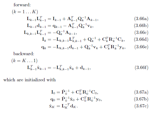
基于cholesky smoother 使用卡尔曼增益,可以将这6个方程改写成 RTS smoother 先验协方差,先验均值,卡尔曼增益,前向后验协方差更新,前向后验均值更新,前向后验均值修正 的形式
这回内容
上一页主要解决上述三四层关系的详细推导,
这一页
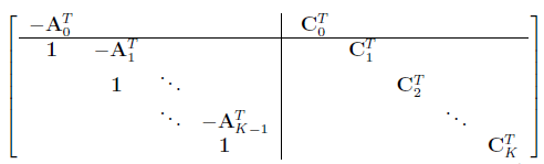
1 关于方程 $(H^{T}W^{-1}H) \hat{x}=H^{T}W^{-1}z$ 何时有解。
2 卡尔曼滤波器的内容。
3.1.4 Existence, Uniqueness, and Observability
$\hat{\mathbf{x}}=\left(\mathbf{H}^{T} \mathbf{W}^{-1} \mathbf{H}\right)^{-1} \mathbf{H}^{T} \mathbf{W}^{-1} \mathbf{z}$
so it has a unique solution if and only if $(H^{T}W^{-1}H) $ is invertible.
and $\mathbf{x}$ is in shape (N(K+1),1) / $\operatorname{dim}{\mathbf{x}} = N(K+1)$ ($x_i \in R^N, \mathbf{x} = [x_0, x_1 … x_k]^T$), so
$\operatorname{rank}\left(\mathbf{H}^{T} \mathbf{W}^{-1} \mathbf{H}\right)=N(K+1)$
and $\mathbf{W^{-1}}$ is invertible and positive definite. so we can drop it. That means
In other words, we need N(K+1) linearly independent rows (or columns) in the matrix $\mathbf{H}^{T}$ .
We now have two cases that should be considered:
(i) We have good prior knowledge of the initial state, $\check{x}_0$.
(ii) We do not have good prior knowledge of the initial state.
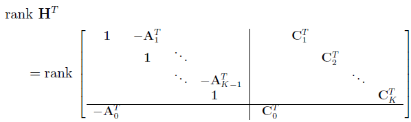
case (i) with initial state
write out $\mathbf{H^T} $ just like in 3.2.2.5. we will find out the matrix is in block-row-echelon from, which means full rank.
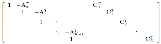
$\operatorname{rank}\mathbf{H^T} = N(K+1)$
and the solution is unique.
case (ii) without initial state
this means remove the first column in $\mathbf{H^T} $
moving the top row to the bottom:
let the $\mathbf{A} $ part of the last row become $\mathbf{0} $ by adding $\mathbf{A_0^T} $ times first row to it, and then $\mathbf{A_0^T}\mathbf{A_1^T} $ times first row ….
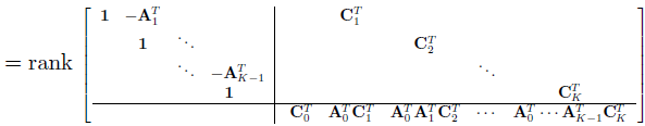
the upper block is full rank of $NK$
so if the bottom block is full rank of $N$, the solution is unique.
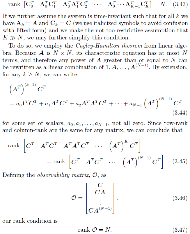
即 可观 = 有唯一解
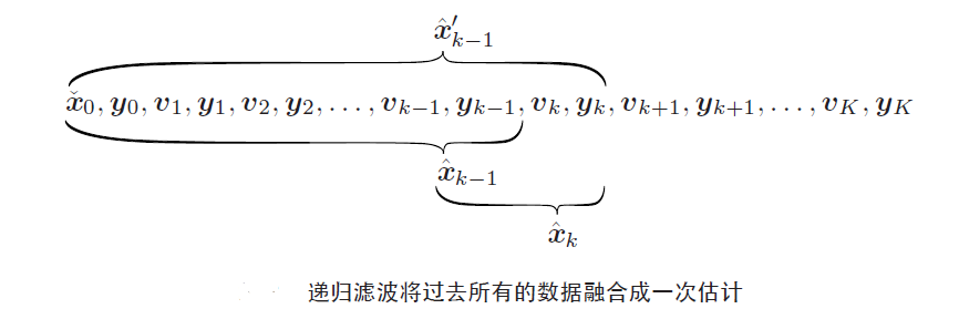
3.3 Recursive Discrete-Time Filtering
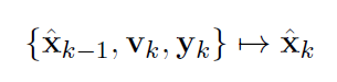
- 递归最小二乘法RLS <RLS和卡尔曼滤波器非常类似> (会用在4中运用)
- RTS的前向部分 即为卡尔曼滤波器 最好先把上一次的RTS看懂
- 经典形式 卡尔曼增益是修正的权重
- 信息形式 信息矩阵是协方差矩阵的逆,即不用卡尔曼增益的形式
- 从MAP出发推导 (即 H W z 简化为 关于 k-1 和 k 时刻 的矩阵, 而非 从0到k时刻的矩阵)
- 从贝叶斯推断出发推导 (不通过HWHx=HWz, 直接从概率出发推导)
- 从gain optimization推导
0. RLS
求J的最小值,就是二次函数最小值,J导=0 得到 xi
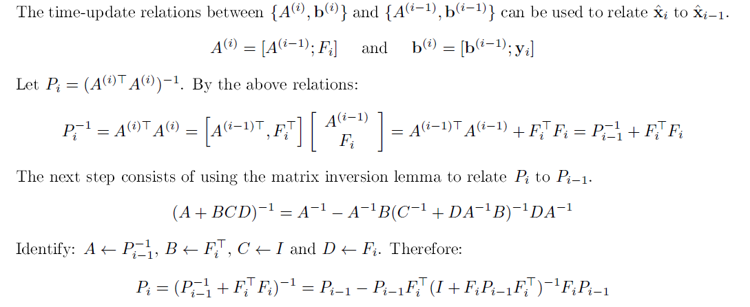
令P的逆等于x中第一项,把其中Ai写成[Ai-1,Fi]的形式,得到Pi的逆递归式。
用SMW恒等式整理(Pi的逆递归式的逆),得到Pi的递归式。
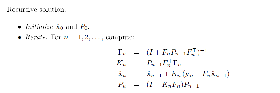
用 Γ, K替换 得到 第4式 Pi
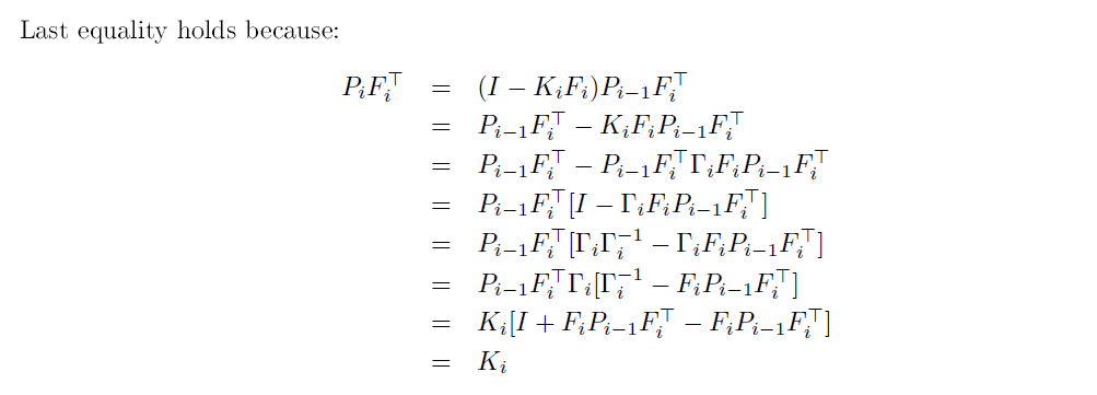
再推导以下Ki和Pi的关系 见下方
第3个式子 xi的推导见下下方
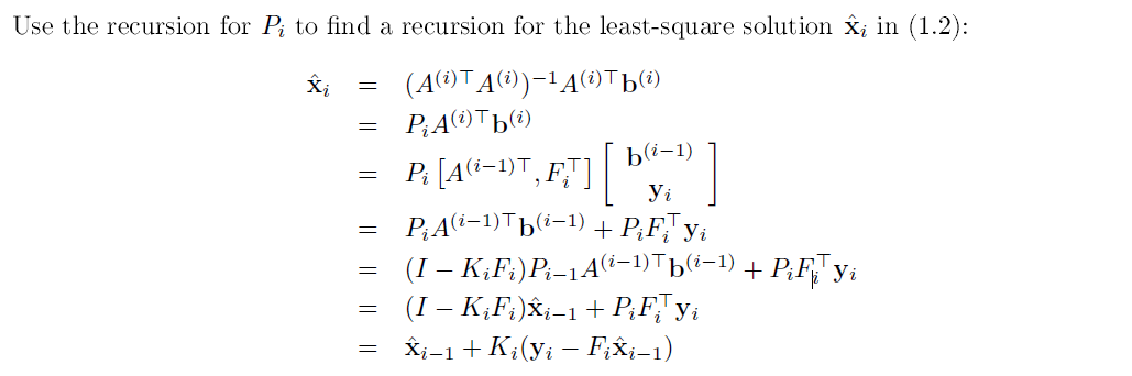
xi 是 最开始得到的结论(1.2)
用之前假设的Pi去替换
把 Ai bi 都拆开,为了递归,并且乘出来
Pi的递归式代入
发现了Pi-1Ai-1bi-1就是1.2中的xi-1 (递归起来了)
代入Ki-Pi的结论 整理
得到递归式
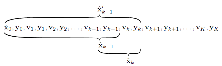
2. MAP
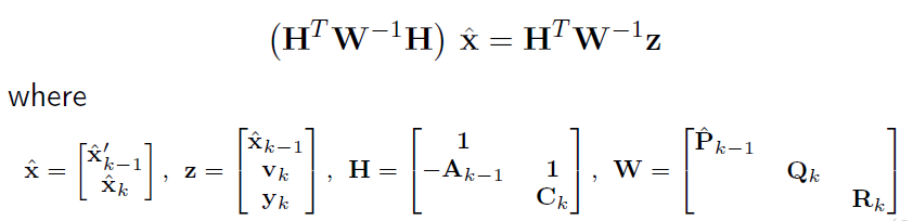
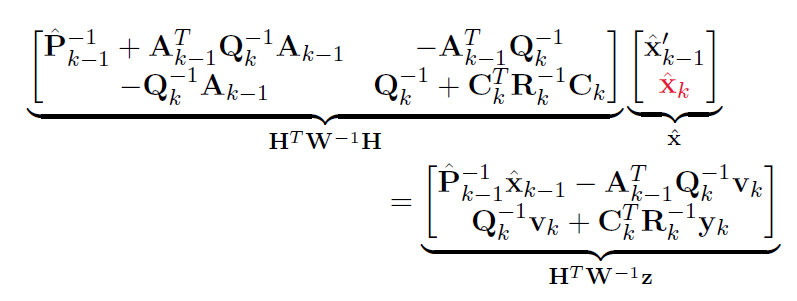
考虑k-1时刻和k时刻的关系
-
代入
-
消去 后验x’k-1
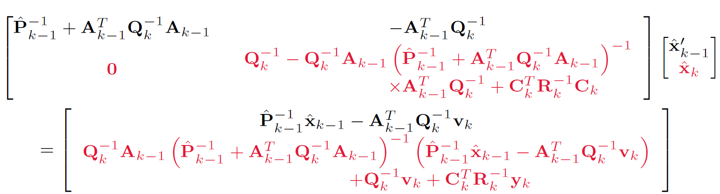
用舒尔补进行消去:
可以直接从Ax+By=a,Cx+Dy=b入手 写出 Ky=d
也可以用求舒尔补的矩阵打洞过程把2,1位置变成0 得到 Ky=d
-
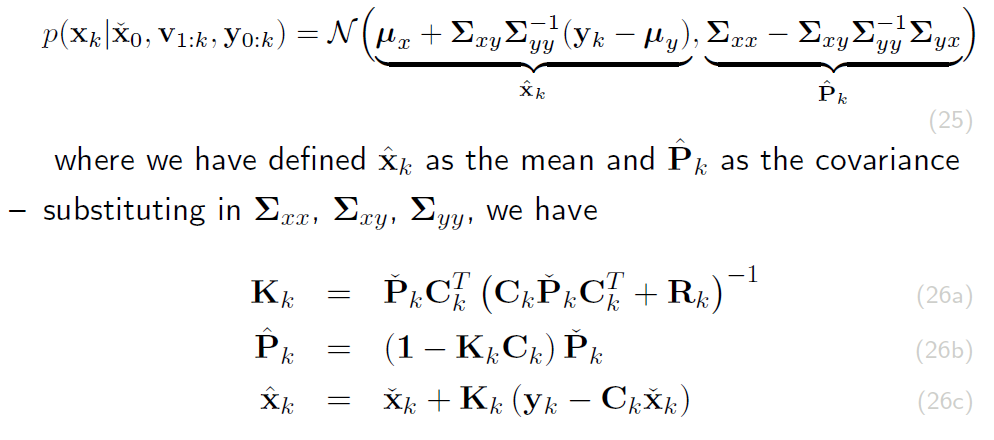
后验xk
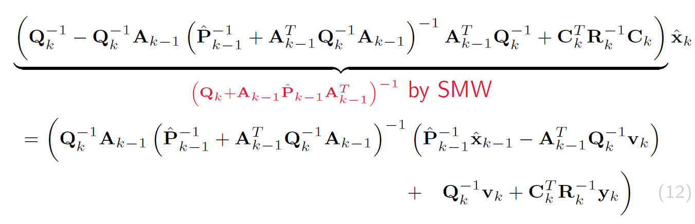
使用的是SMW第一式
-
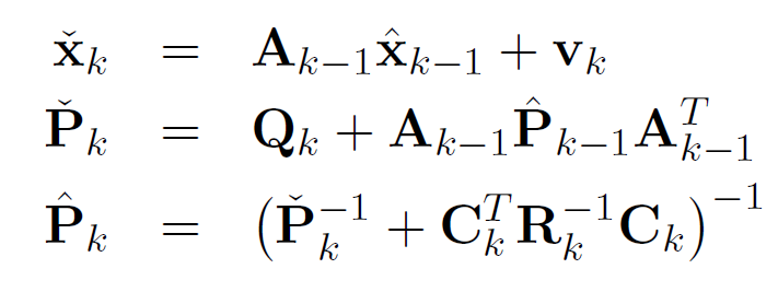
定义 先验xk,先验Pk,后验Pk
-
代入得到
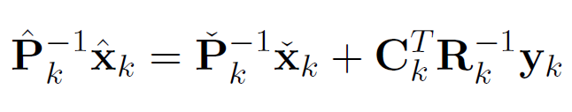
即
信息形式的RTS前向部分 -
加入卡尔曼增益 K
具体方法可以看上一次的RTS部分。这边有很多代入方法。
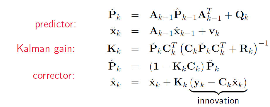
得到
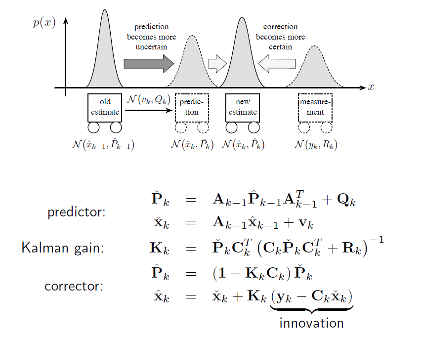
经典形式的卡尔曼滤波器意义:
-
k-1时刻的后验 – system dynamics -> k时刻的先验:
是根据 输入 和 k-1时刻的估计状态 做出的猜测
输入 input v
输入噪音 process noise w ~ N(0,Q)
-
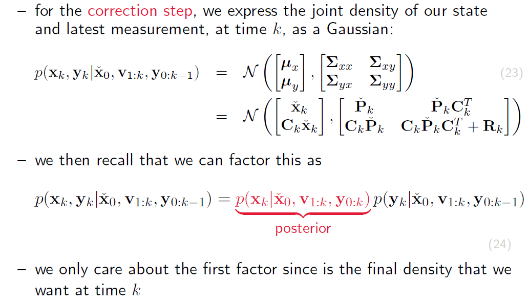
k时刻的先验 – measurment model -> k时刻的后验:
是根据 测量 和 k时刻的猜测 做出的最后修正估计结果
测量 mesurment y
测量噪音 mesurment noise n~ N(0,R)
y-Cx 是实际测量和理论测量的差 = 一个修正
卡尔曼增益 kalman gain :
how much you want to take the prediction in account. if R is very large, so the measurement is very uncertain, so we get a smaller K. that means we don’t trust the measurement.
协方差:与输入和测量无关,所以每次都只需要求均值即可。
-
3. Bayesian Law
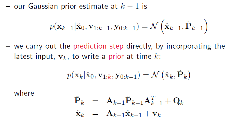
先算Prior
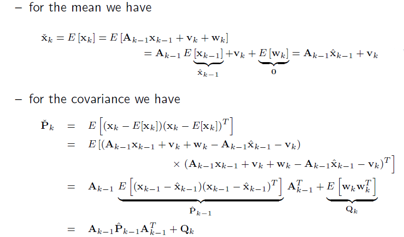
先验均值,和上一回的时候一样的做法,简化一下。
先验协方差,和上回测量协方差的步骤差不多。
下图
k-1时刻: 在 一串到k-1时刻的输入和测量 条件下的 计算 就是估计 是 后验k-1
k时刻: 比上一个k-1多了一个k时刻的输入 这时的计算 是猜测 是先验k
k的先验和MAP中一样
然后算Joint Probability 和上一次一样
接着是用高斯推断算Posterior 和上次一样
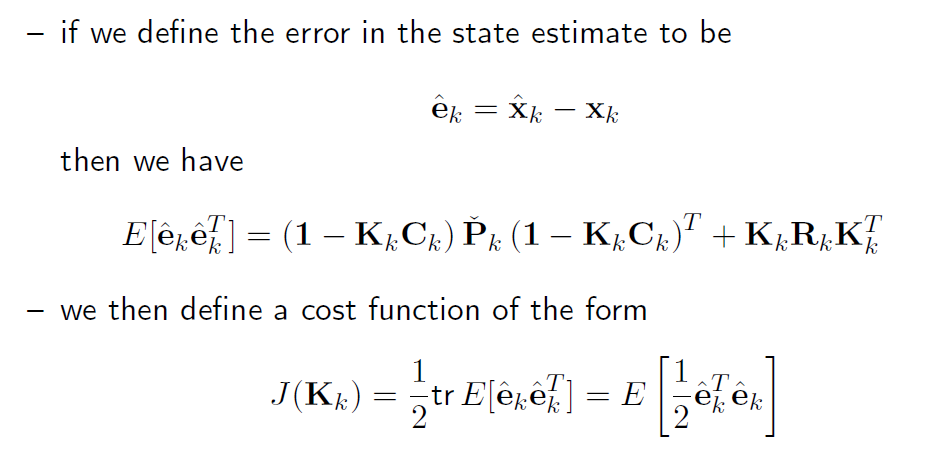
4. Gain Optimization
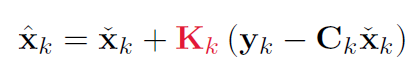
假设 后验(修正过的估计) 是 先验(猜测) + 修正(测量修正) * 修正的比例(K)
也就是我们先假设了 后验xk = 先验xk + Kk(yk-Ck*先验xk) 这个式子
然后我么找最合适的K
用cost function
先定义偏差时 后验x(修正过的估计) - 实际

卡尔曼滤波器
最优线性无偏估计(BLUE)
总结
Smoother
- Batch Discrete-Time Estimation (得到方程,用线性代数的方法解方程)
- MAP
- 贝叶斯
- Recursive Discrete-Time Smoothing (用recursive的方法求解方程)
- Cholesky
- RTS
Filter
- Recursive Discrete-Time Filtering
- KF
SER目录
| SER目录 | ||
|---|---|---|
| SER-1 | K2 - 基础概率论 | |
| SER-2 | K3 - LG系统下Batch/Smoother | |
| SER-3 | K3 - LG系统下Recursive Filter | |
| SER-4 | K4 - NLNG系统下Recursive Filter | |
| SER-5 | K4 - NLNG系统下Batch | |
| SER-6 | K5 - 偏差,匹配和外点 |