Robotics inherently deals with things that move in the world.
Introduction
Common Issues in applications:
- State estimation
- State: a set of quantities (position, orientation, velocity, …)
- Control
Sensors and Measurements
interoceptive: measurements of velocity, acceleration- eg. accelerometer, gyroscope, wheel odometer
exteroceptive: measurements of position, orientation- eg. camera, time-of-flight transmitter/receiver(laser rangefinder, GPS)
Problem in this book: Estimation is the problem of reconstructing the underlying state of a system given a sequence of measurements as well as a prior model of the system.
状态估计,是根据系统的先验模型和测量序列,对系统内在状态进行重构的问题。
Estimation Machinery
K2 Primer on Probability Theory
重点就是 2.2.3高斯推论,2.2.5高斯分布线性变换 **和 **2.2.8高斯分布非线性变换。
2.1 PDF
这一章节主要是一些基础概率论公式。
因为最后要笔试,所以写得稍微详细一点,以免到时候突然卡壳。其实基本上不用怎么看,可以直接跳到 2.1总结 。
2.1.1 Definitions
probability: $\int_a^b p(x)dx = 1$
conditional probability: $(\forall y) \int_a^b p(x \mid y)dx = 1$
joint probability: $\int_a^b p(x)dx =\int_{a_N}^{b_N}…\int_{a_2}^{b_2}\int_{a_1}^{b_1}p(x_1,x_2, … ,x_N)dx_1dx_2…dx_N = 1$
2.1.2 Bayes’ Rule and Inference
$p(x \mid y) = $ $\frac{p(y \mid x) \cdot p(x)}{p(y)} $
物理意义: $x$ := 状态,$y$ := 传感器读数,$p(y|x)$ := 传感器模型,$p(x|y)$ := 状态估计
离散的类推:参考高中数学/概率论:
介于生活离开数学已经有段时间了,这里用wiki的吸毒者检测范例回顾一下:
$x$:= 吸毒, $\bar x$:= 不吸毒, $y$:= 阳性, $\bar y$:= 阴性
吸毒率预计为0.5%,则 $p(x)$=0.005 , $p(\bar x)$ = 0.995 , 为x的先验概率(prior)。
检测试剂的阳性检测准确率(Sensitivity),即吸毒的人被检查出阳性的概率为99%,则 $p(y|x)$=0.99 ,是似然(Likelihood);出错率则为1%,即 $p(\bar y|x)$=0.09 。检测试剂的阴性检测准确率(Specificity),即不吸毒的人被检查出阴性的概率为99%,则 $p(\bar y|\bar x)$=0.99 ;出错率则为1%,即 $p(y|\bar x)$=0.09 。
那么阳性检出率,即一个人吸毒且被查为阳性 或 不吸毒且被查为阳性,$p(y)= p(x,y) + p(\bar x,y) = p(x) \cdot p(y|x) + p(\bar x) \cdot p(y|\bar x)$ = 0.0149 ,是y的边缘概率/标准化常量。
那么对于一个呈阳性的人,他真的吸毒的概率 $p(x|y) = \frac{p(y | x) \cdot p(x)}{p(y)} $ = 0.3322, 即已知y发生后x的条件概率/x的后验概率(posterior)。
返回到状态估计理论:即在传感器读数y成阳性的条件下,估计x的吸毒史状态。
by marginalization:
$ = \int p(x,y)dx = \int p(y\mid x)\cdot p(x)dx$
边缘概率:传感器读数是0.1的概率有多大 p(y=0.1) = 求和所有p(x 且 y=0.1)组合。
2.1.3 Moments
- zeroth probability: 1
- first probability:
mean$\mu = E[x]=\int xp(x)dx$ - second probability:
covariance matrix$\Sigma = E[(x-\mu)(x-\mu)^T]$
2.1.4 Sample Mean and Covariance
expected: mean $\mu$, covariance$\Sigma$
approach: sample mean $\mu_{meas} $, sample covariance $\Sigma_{meas}$(with (N-1) as Bessel’s correction)
Bessel’s correction
假定:$\mu$ 已知,$\Sigma$ 未知,则:$\Sigma = E[\frac{1}{n}\sum_1^n(x_i-\mu)^2]$
现实:$\mu$ 未知,$\Sigma$ 未知,用样本均值 $\mu_m $ 代替 $\mu$ 会导致 $E[\frac{1}{n}\sum_1^n(x_i-\mu_m)^2] < E[\frac{1}{n}\sum_1^n(x_i-\mu)^2] = \Sigma$,导致 $\Sigma$ 被低估, 所以需要用 (n-1) 放大一些。详细证明,见知乎 - 马同学的回答。
2.1.5 Statistically Independent, Uncorrelated
Independent$p(x,y) = p(x)p(y)$Uncorrelated$E[xy^T]=E[x]E[y]^T$
相关系数 $r = \frac{Cov(x,y)}{\sigma_x\sigma_y}$ 可以看作是标准化后的协方差,剔除了变量变化幅度对相关性的影响。从几何的角度,一定程度上,协方差可以理解为向量x,y的内积,相关系数是夹角的余弦值。
$r = 0$ 表示 uncorrelated, 即 $cov(x,y) = E[(x-\mu_x)(y-\mu_y)] = E[xy-\mu_xy-x\mu_y+\mu_x\mu_y]$ $=E[xy]-\mu_xE[y]-\mu_yE[x]+\mu_x\mu_y = E[xy]-\mu_x\mu_y-\mu_x\mu_y+\mu_x\mu_y = E[xy]-E[x]E[y] = 0$
Independent $\rightarrow$ Uncorrelated, but Uncorrelated $\nrightarrow$ Independent .
eg. $x^2 + y^2 = 1$
In Gaussian distribution: Independent $\equiv$ Uncorrelated
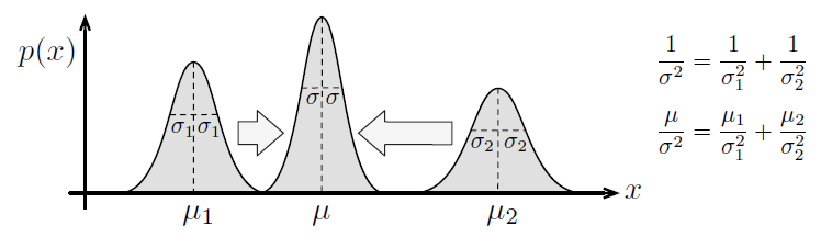
2.1.6 Normalized Product
merge two estimations (eg. from different sensors) $p_1(x), p_2(x)$ as $p_1(x) \cdot p_2(x)$, search an $\eta$
if $x$ is a status, $y_1$ and $y_2$ are two measurements from two statistical independent sensors:
$p(x \mid y_1, y_2) =$ $\frac {p(y_1,y_2 \mid x)p(x)} {p(y_1, y_2)}$ $\tag{Bayes' Rule [2]} $ $p(y_1,y_2 \mid x) = p(y_1 \mid x)p(y_2\mid x)= $$\frac{p(x\mid y_1)p(y_1)} {p(x)}\frac{p(x\mid y_2)p(y_2)}{p(x)}$ $\tag{Independence and Bayes' Rule [3]}$ $p(x \mid y_1, y_2) = p(x\mid y_1)p(x\mid y_2)$$\frac{p(y_1)p(y_2)} {p(y_1,y_2)p(x)}$$\tag{[3]+[2] [4]}$
Compare [4] and [1], $\eta = $$\frac{p(y_1)p(y_2)} {p(y_1,y_2)p(x)}$. So if $p(x)$ is uniform over all values of x (i.e., constant), then is $\eta$ also a constant.
2.1.7 Shannon and Mutual Information
-
Negative Entropy(Shannon information): $H(x) = -E[\ln{p(x)}] = - \int p(x) \ln{p(x)}dx$ -
Mutal Information: $I(x,y) = E[\ln{\frac{p(x,y)}{p(x)p(y)}}] = \int \int p(x,y) \ln(\frac{p(x,y)}{p(x)p(y)})dxdy$
Clearly, if x,y are independent, $I(x,y) = 0$. Else, $I(x,y) = H(x)+H(y)-H(x,y)$.
2.1.8 Cramér-Rao Lower Bound and Fisher Information
2.1 小结
| 普通的概率密度函数 | |
|---|---|
| 定义和关系 | 联合 = 条件$ \times $边缘 |
| 贝叶斯 | 后验 = $ \frac{似然 \times 先验}{标准化常量}$ |
| 矩 | 期望、方差 以及 与样本均值、样本方差的区别 |
| 独立/不相关 | 定义 |
| 归一化积 | 定义、原理 |
| 信息熵 | 负熵、互信息 及 其关系: 互信息 = 边缘熵之和 - 联合熵 |
我以为这是一门有意思的课 :) , 没想到又是数学课。暴毙。
2.2 Gaussian PDF
这一章节是看高斯密度函数的一些基本性质。线代+概率论
这里仅做初步整理。
重点是:高斯推论 以及 线性/非线性变换。
2.2.1 Definitions
-
Gaussian PDF: $p(x\mid\mu,\sigma^2)=$$\frac{1}{\sqrt{2\pi\sigma^2}}$$exp(-$$\frac{1}{2}\frac{(x-\mu)^2}{\sigma^2})$-
Q1: $\int p(x) dx= 1$ ?
-
-
multivariate Gaussian PDF: $p(x\mid\mu,\Sigma)=$$\frac{1}{\sqrt{(2\pi)^Ndet(\Sigma)}}$$exp(-$$\frac{1}{2}$ $(x-\mu)^T \Sigma^{-1}(x-\mu))$-
mean$\mu = E[x] =\int_{-\infty}^{\infty}xp(x)dx$ -
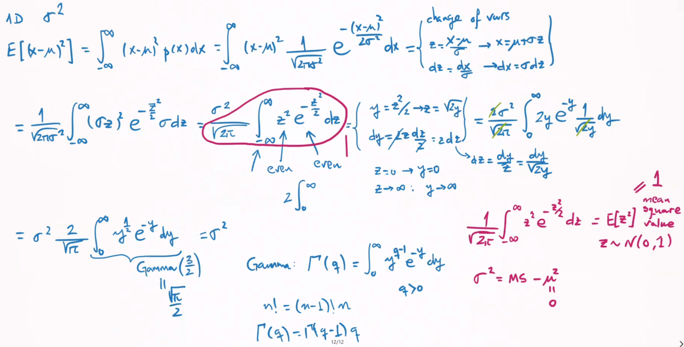
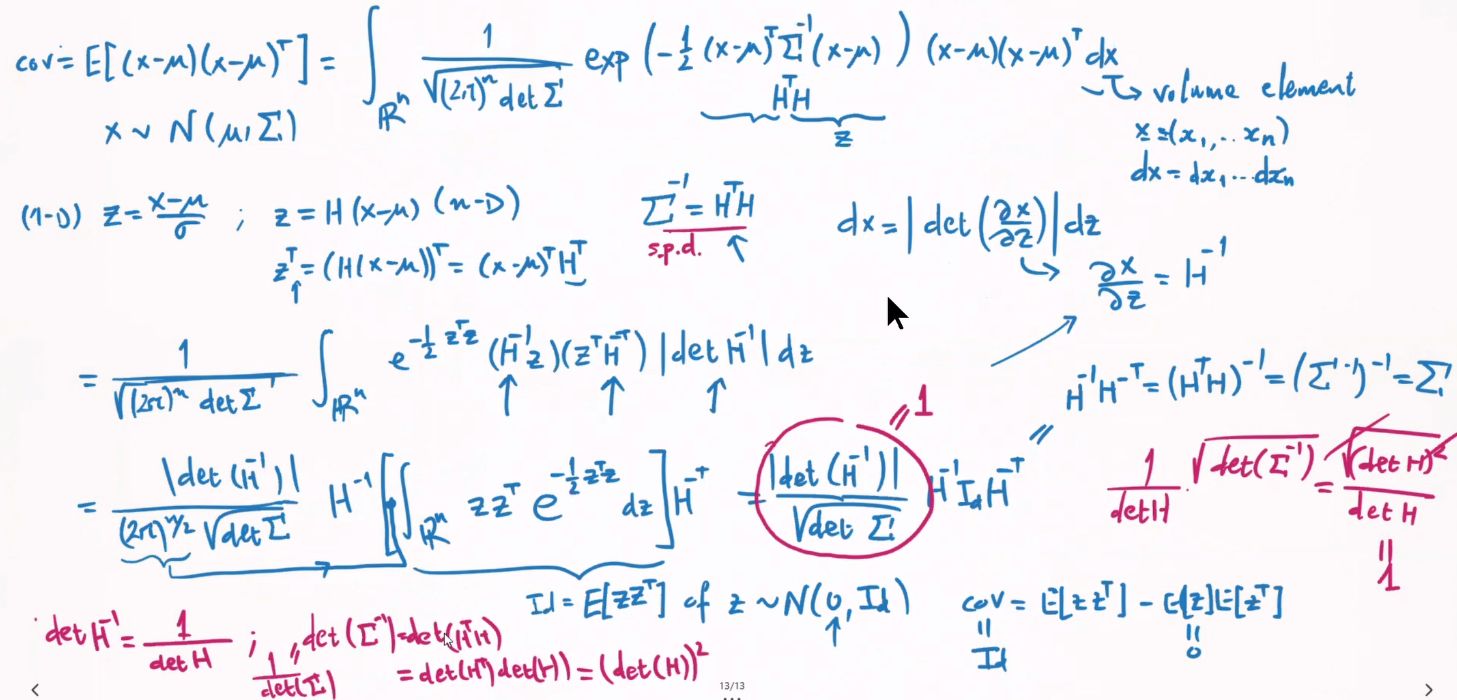
covariance matrix$\Sigma = E[(x-\mu)(x-\mu)^T] = \int_{-\infty}^{\infty}(x-\mu)(x-\mu)^Tp(x)dx$ -
物理意义:$\mu$ 最高点的位置 , $\Sigma$ 等高线(椭圆)的情况
-
Q2: from
Gaussian PDFtomultivariate Gaussian PDFQ3:
mean$\mu$ andcovariance matrix$\Sigma$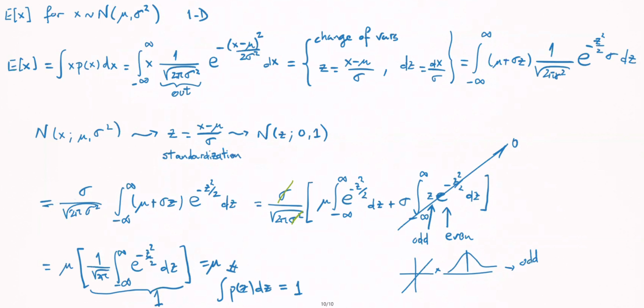
-
2.2.2 Isseris’ Theorem
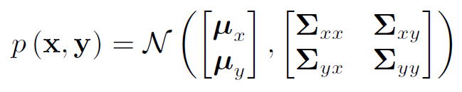
2.2.3 Joint G-PDF
Q4:
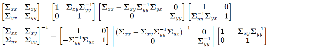
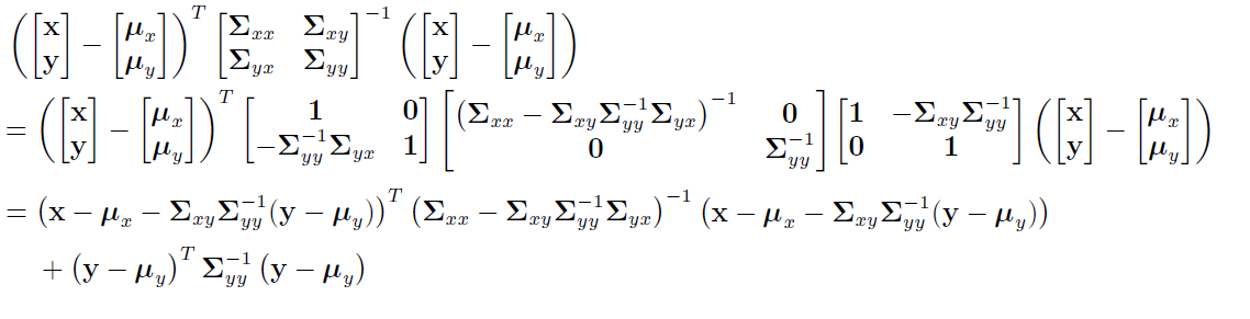
Gaussian inference: $p(y)$ and $p(x \mid y)$Covariance matrix in UDL-Decomposition or Schur-Complement:
Exponent part of Gaussian PDF:
so: $p(x,y) = p(x|y)p (y)$
2.2.4 Statistically Independent, Uncorrelated
Independent $\equiv$ Uncorrelated
Q5: Independent $\equiv$ Uncorrelated
2.2.5 Linear Change
$x \in \mathbb{R} ^ N \sim \mathcal{N}(\mu_x, \Sigma_{xx})$
if $y = Gx$ with $G \in \mathbb{R} ^ {M \times N}$
mean$\mu_y = E[y] = E[Gx] = G\cdot E[x] = G\mu_x$covariance matrix$\Sigma_{yy} = E[(y-\mu_y)(y-\mu_y)^T] = G \cdot E[(x-\mu_x)(x-\mu_x)^T] \cdot G^T = G\Sigma_{xx}G^T$
So $y \sim \mathcal{N}(\mu_y, \Sigma_{yy}) = \mathcal{N}(G\mu_x, G\Sigma_{xx}G^T)$
Q6: Another way?
2.2.6 Normalized Product
Q7: Proof
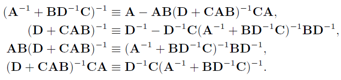
2.2.7 Sherman-Morrison-Woodbury Identity
简单的矩阵分解,将用于高斯分布的非线性变换。
$ M = \left[ \begin{matrix} A^{-1} & -B \\\ C & D \end{matrix} \right] $
Reform M into LDU and UDL.
Invert M based on these 2 forms. That is: $M^{-1}=(LDU)^{-1}=(UDL)^{-1}$
Unfold and compare $(LDU)^{-1}, (UDL)^{-1}$
2.2.8 Nonlinear Change
That is to calculate p(y):
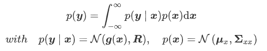
Linearization of $\mathbf{g(\cdot)}$:
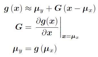
非线性变换 $g(\cdot)$后 $\mu_y$不一定等于 $g(\mu_x)$ (只有线性变换才肯定等于)。这边是假设。
然后对$x=\mu_x$点取偏导,即Jacobi矩阵。即 线性化该模型 $g(\cdot)$。
现在 $g(\cdot)$ 是一个线性变换了,那么再代回 $p(y)$。
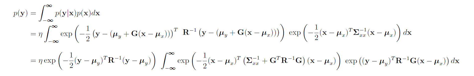
为什么这么变形:
因为都有 $y-\mu_y$,而且是对 $x$做积分,想到拆分无关的 $y$部分。
接下来如何变形:
那么现在积分内的部分,相当于 $a^2 - 2ab$ ($a = x-\mu_x, b=y-\mu_y$,实数系数 $-1/2$接下来不考虑了)。那么想到补全平方项 $(a- b)^2 -b^2$。比较系数(即矩阵部分), $a^2$前是 $\Sigma_{xx}^{-1}+G^TRG$, $2ab$前是$R^{-1}G$,定义一个 $F$使整理方便。
令 $F^T \cdot (\Sigma_{xx}^{-1}+G^TRG )= R^{-1}G$, 为了简明 这边再令 $A = \Sigma_{xx}^{-1}+G^TRG$,以及省略矩阵乘法的转置等操作。
那么 原式 = $A\cdot a^2 - 2\cdot FA\cdot ab = A(a-F\cdot b)^2-F^2\cdot b^2$。最后还有一开始的$-1/2$。
下图第一行是完全平方部分,第二行是$F^2b^2$部分。
积分部分
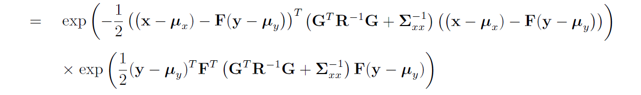
接下来又要干嘛:
第一部分是关于 $x$的积分,而我们需要 $p(y)$,根据全概率公式,积完后得到常数,可以与 归一化积 $\eta$合并。
第二部分$F^2b^2$,即 $(y-\mu_y)$的部分,与 $x$无关, 提出积分,也是最后剩下的部分。
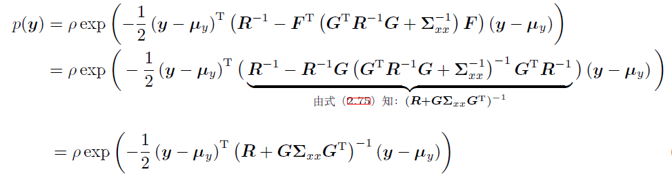
根据 $F^T \cdot (\Sigma_{xx}^{-1}+G^TRG )= R^{-1}G$,替换回 $F$。
然后根据SMW恒等式,观察后….,即可化简。
最后得到关于y的高斯分布。
2.2.9 Shannon Information of GPDF
2.2.10 Mutual Information of GPDF
2.2.11 Cramer-Rao Kower Bound of GPDF
2.2 小结
| Gaussian PDF | ||
|---|---|---|
| 定义和关系 | 联合 = 条件$ \times $边缘 | 一维 → 多维 高斯推断:联合 → 条件、边缘 |
| 贝叶斯 | 后验 = $ \frac{似然 \times 先验}{标准化常量}$ | |
| 矩(线性变换) | 期望、方差 | 线性变换 |
| 独立/不相关 | 定义 | 证明 |
| 归一化积 | 定义、原理 | 证明 (像并联电路电阻) |
| 信息熵 | 负熵、互信息 互信息 = 边缘熵之和 - 联合熵 |
*<略>* |
| CR下界 | *<略>* | *<略>* |
| 其他 | 非线性变换(线性化) |
SER目录
| SER目录 | ||
|---|---|---|
| SER-1 | K2 - 基础概率论 | |
| SER-2 | K3 - LG系统下Batch/Smoother | |
| SER-3 | K3 - LG系统下Recursive Filter | |
| SER-4 | K4 - NLNG系统下Recursive Filter | |
| SER-5 | K4 - NLNG系统下Batch | |
| SER-6 | K5 - 偏差,匹配和外点 |