Estimation Machinery
分成了
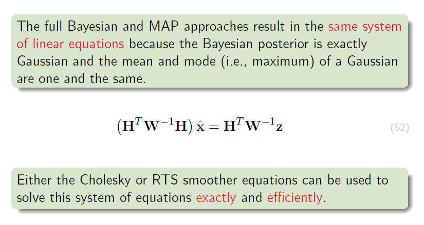
线性高斯系统(LG)和非线性非高斯(NLNG)系统 分别在K3 K4分析。这一页主要涉及LG系统下,通过MAP和贝叶斯推断,以及Cholesky smoother和RTS smoother 详细求解
运动方程及观测方程的过程。
K3 Linear-Gaussian Estimation - 1
3.1 Batch Discrete-Time Estimation
3.1.1 Setup
for linear, time-varying models: we need
a motion model and a observation model:
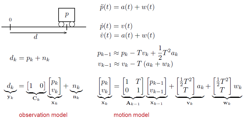
So 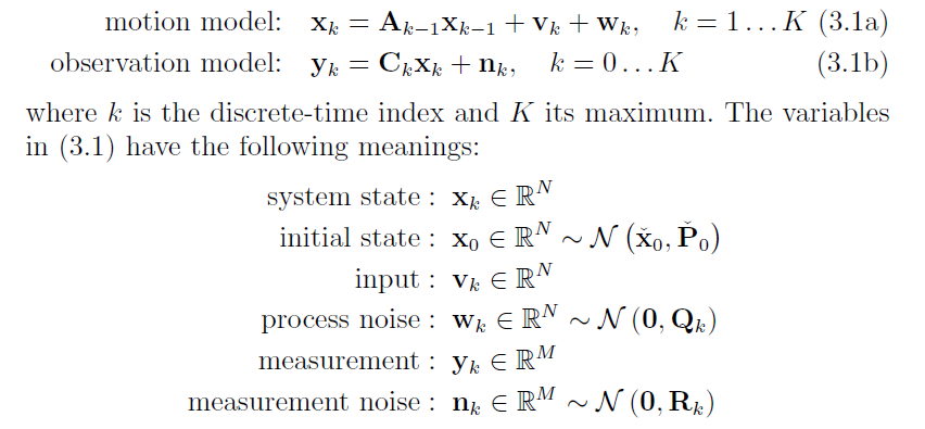
分成
batch linear-Gussain techniques (smoothers)和recursive state estimators (filters)分别在3.1.2 MAP + 3.1.3 Bayesian 和 3.3 Kalman Filter
即求解: $\hat{x}$ (posterior) 后验的协方差和均值.
3.1.3 Bayesian inference
Base on the Bayesian Rule with joint & condition:
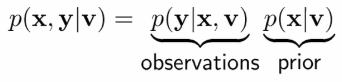
we calculate the prior and the observation to get the joint.
change x and y:
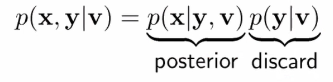
now based on the Gaussian Inference we can use joint to infer posterior
-
For the Prior:
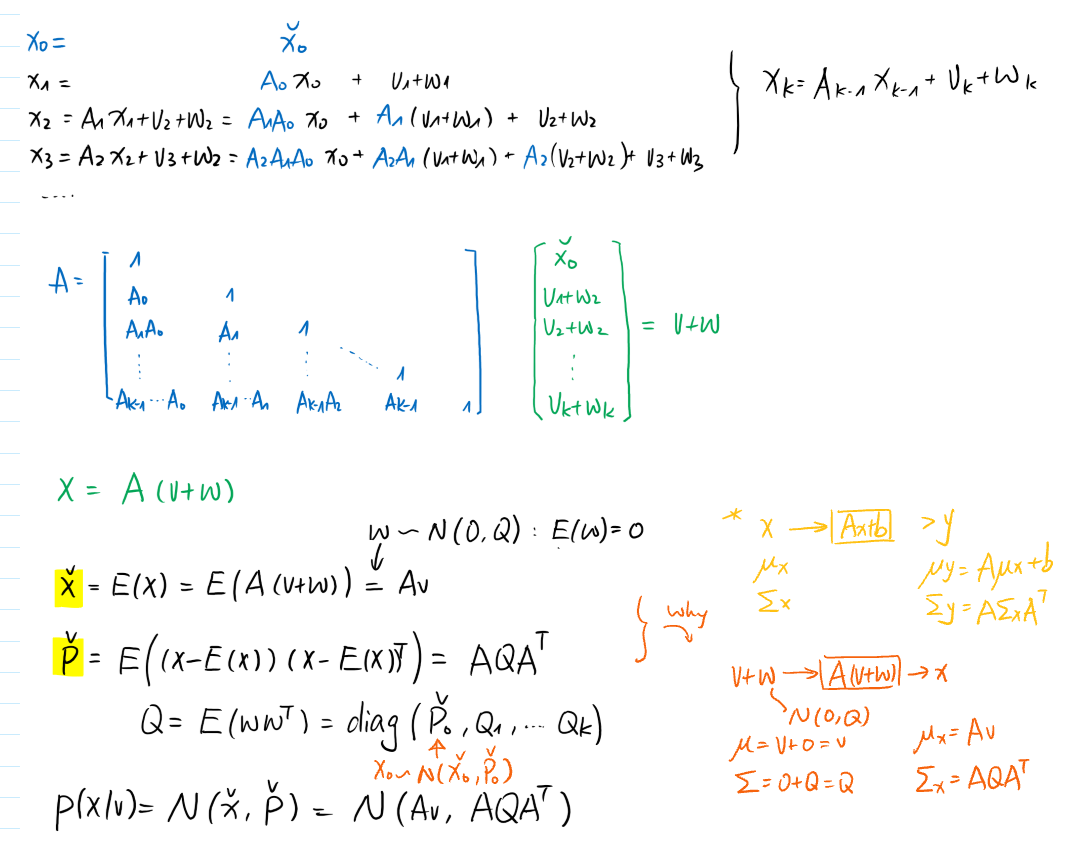
-
For the Observation:
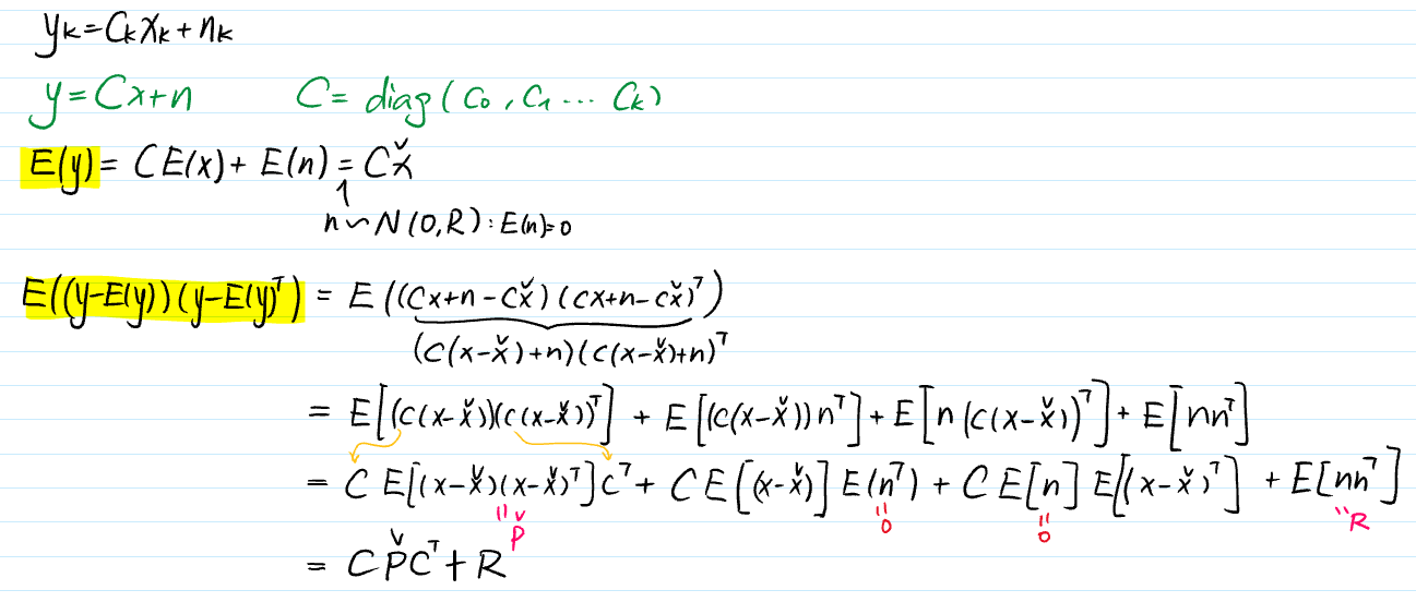
-
For the Joint:
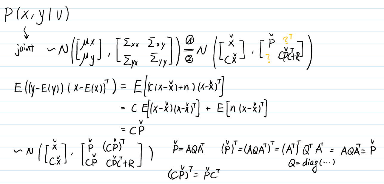
-
For the Posterior:
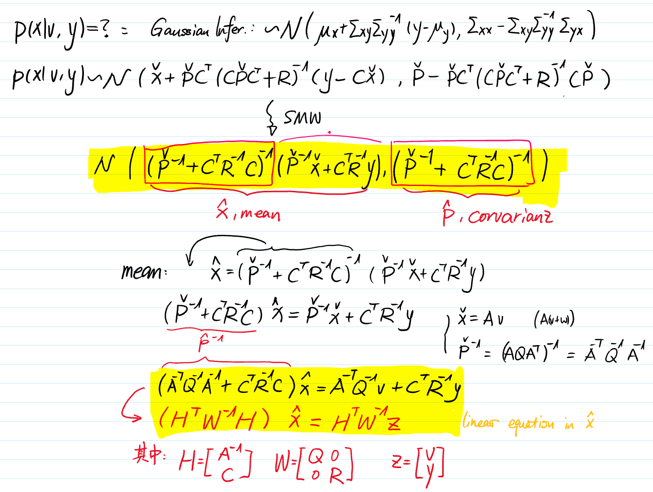
3.1.2 Maximum A Posteriori (MAP)
in batch estimation is to solve:

with Bayes’ rule: <same as in 3.1.3>

by assuming noise variables are uncorrelated:
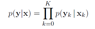
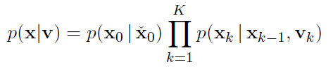
using log function to convert × into +:
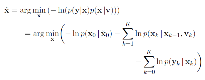
the component parts are:
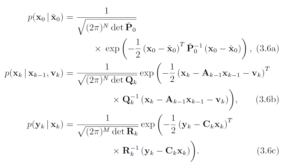
here for example:
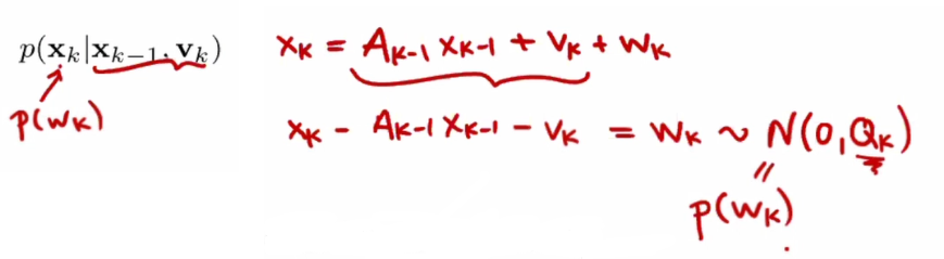
give them into a log function:
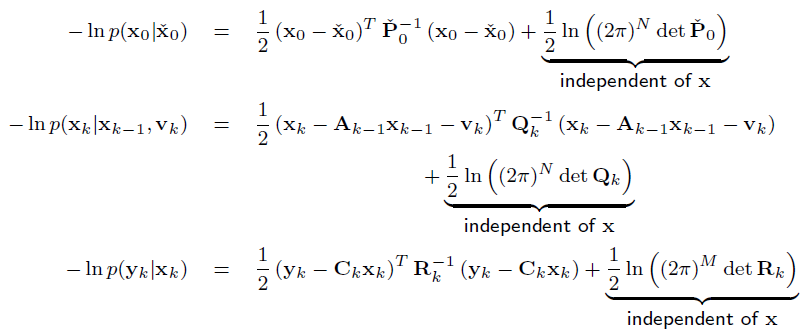
merge them together to get a cost function J(x):
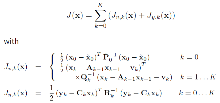
the same as 3.1.3.(4), rewrite the cost function in matrix way:
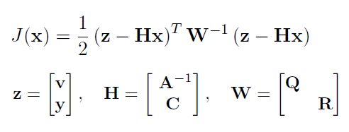
now we calculat the x which reaches the minimum of J:
we found that J(x) is a quadratic function:
对于一维二次函数 找最小值就是 一阶导数等于0,二阶导数大于0。
对于高维二次函数 同理:
先对 f(x+Δx)进行高维泰勒展开如图:
泰勒展开的前两项相当于在操作点附近做线性拟合(雅可比矩阵),前三项相当于在操作点附近做二次函数拟合(海塞矩阵)。
再对x+Δx 代入 f(x)进行展开
比较系数可得泰勒展开中,Δx前的系数即为x的偏导数。
那么如果 f(x)是:
也就是最小二乘问题


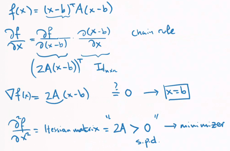
so
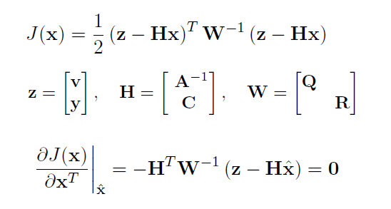
we get the exact equation as in 3.1.3.(4)
3.2 Recursive Discrete-Time Smoothing
3.2.2 Cholesky Smoother
to solve the equation:
-
$A$ and $A^{-1}$
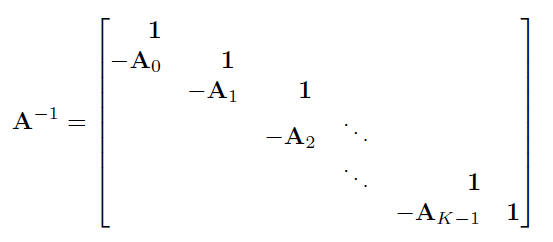
1 下三角矩阵求逆
2 Markov property
-
$H^TW^{-1}h$
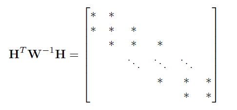
-
using cholesky decomposition : $H^TW^{-1}h = LL^T$ with
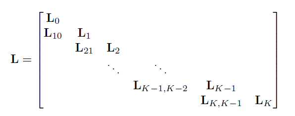
-
reform
$(H^{T}W^{-1}H) \hat{x}=H^{T}W^{-1}z$
$LL^T\hat{x}=H^{T}W^{-1}z$
$Ld=H^{T}W^{-1}z$ with $L^T\hat{x}=d$
-
solve
solve $Ld=H^{T}W^{-1}z$ for $d$ forward
solve $L^T\hat{x}=d$ for $x$ backward
$H = \left[ \begin{matrix} A^{-1} \\\ C \end{matrix}\right] \qquad A \& A^{-1} (step 1) \qquad C = diag(…)$
$H^T = \left[ \begin{matrix} A^{-T} C^T \end{matrix}\right]$
$W = \left[ \begin{matrix} Q & \\\ & R \end{matrix}\right] \qquad Q = diag(…) \qquad R= diag(…) $
$W = diag(w_0,w_1,…)$
$W^{-1} = diag(w_0^{-1},w_1^{-1},…)$
$H^TW^{-1}H$展开乘出来
总结:
- 解HWH=LL 得到L
- 解Ld=HWz 得到d
- 解Lx=d 得到x
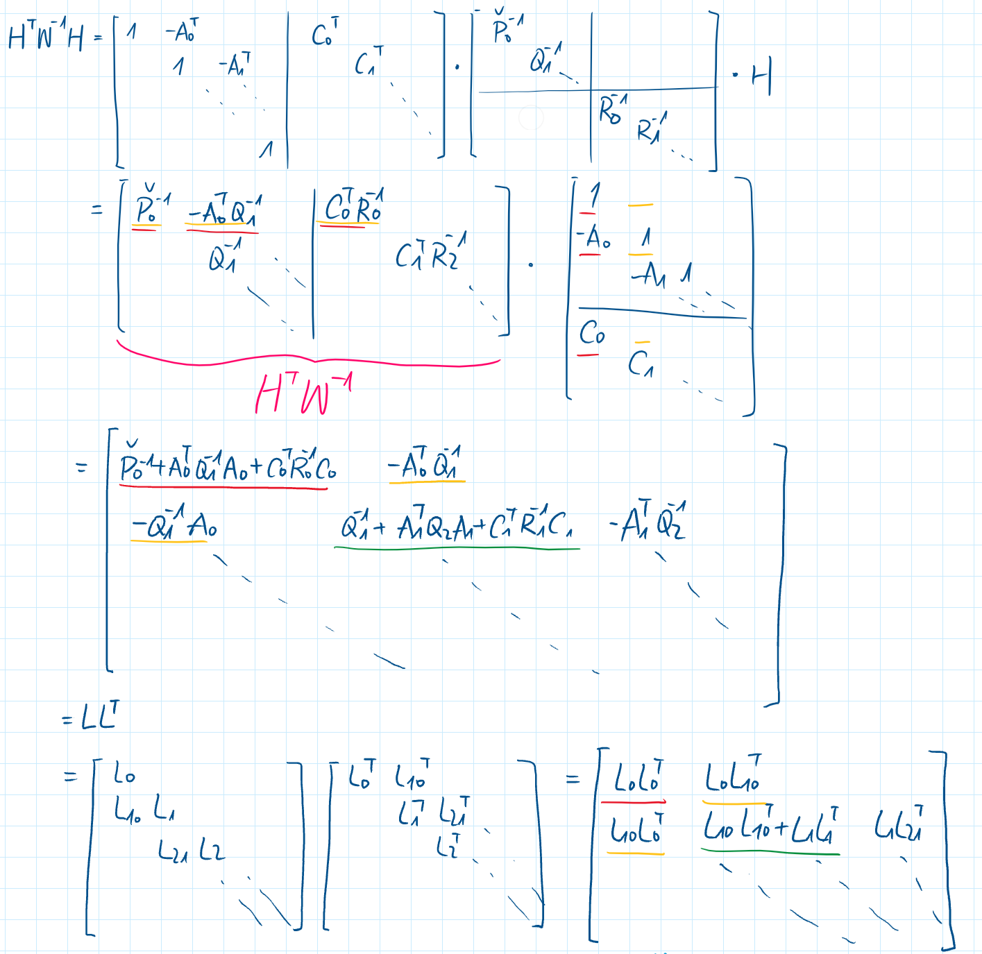
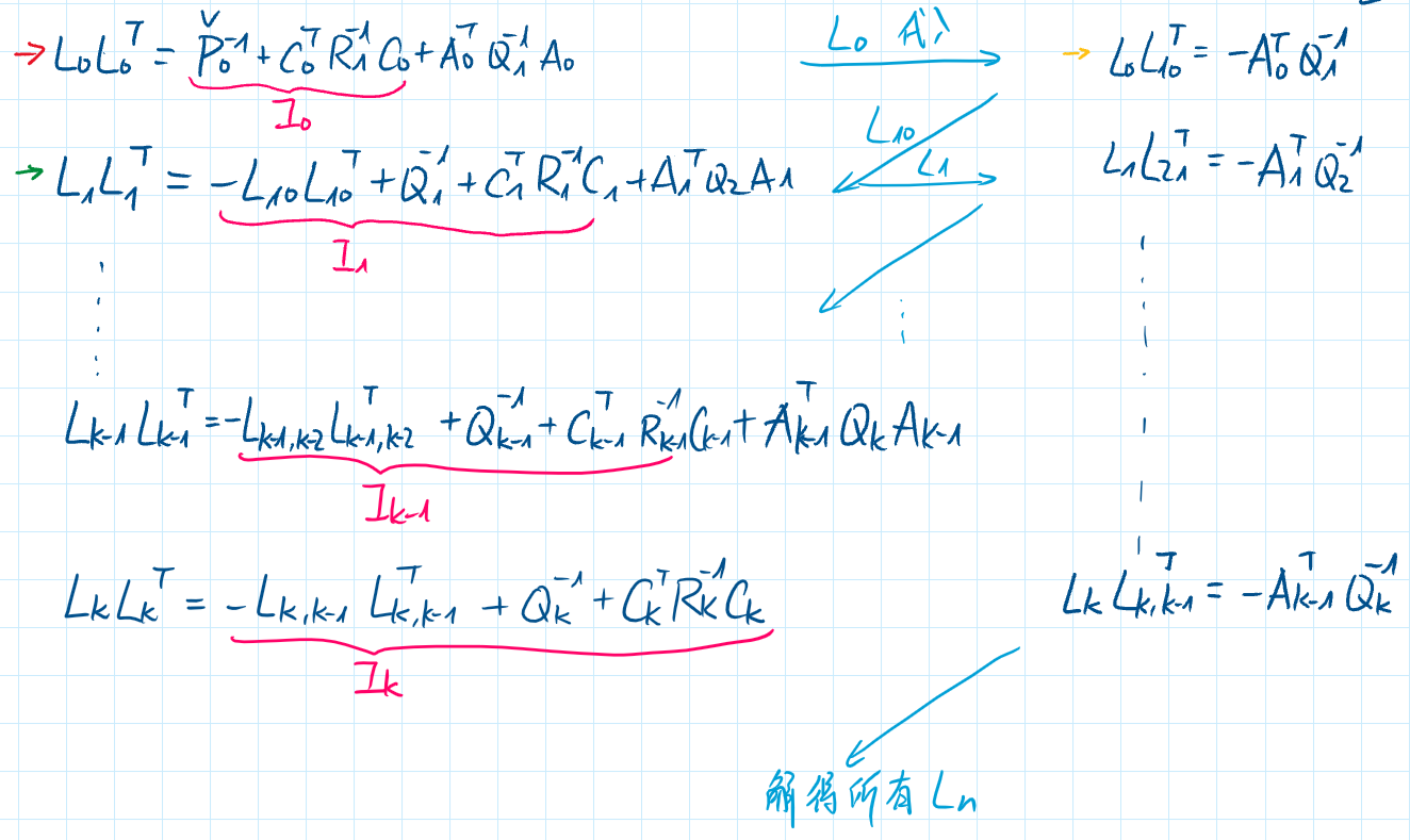
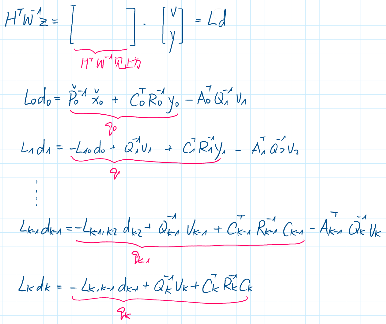
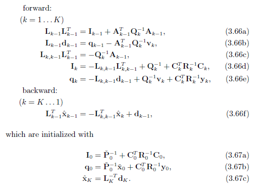
等价于RTS-smoother, 其中前五个前向迭代等价于卡尔曼滤波器
3.2.3 Rauch-Tung-Striebel (RTS) smoother
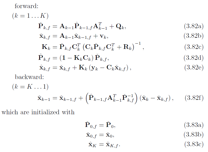
整个RTS由5+1个式子+3个初始状态构成:(1-5由前向得到,6由后向得到)
先观察5个前向迭代的式子 3.66a-3.66e:
A. 后验协方差部分
-
由c式解出 $L_{k,k-1}$,代入d式,化简过程中出现a式再代入:

-
使用SMW化简,得到 $I_k$的递推表达式:

$I$即
信息矩阵information matrix。信息矩阵是协方差的逆。 -
令 $\hat{P}_{k,f} = I_k^{-1}$ (其中 $f$代表forward),则:(这么设是因为信息矩阵的逆是协方差矩阵)
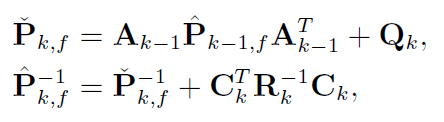
第一个式子代表
先验/预测的协方差第二个式子代表
后验/修正的协方差 (4-5进一步用卡尔曼增益变形该式)即代表:
用k-1的后验预测得到k的先验,在通过k的先验修正成k的后验。(这个过程就是卡尔曼滤波过程)
-
令 $K_k = \hat{P}_{k,f}C_k^TR_k^{-1}$,并将第二式代入K消去后验, 并使用SMW变换:(这么设是因为要写成经典形式,K是卡尔曼增益)

即可通过先验求得K
-
那么根据第二式:


协方差更新方程:即后验协方差对先验协方差的更新/修正
B. 均值部分
-
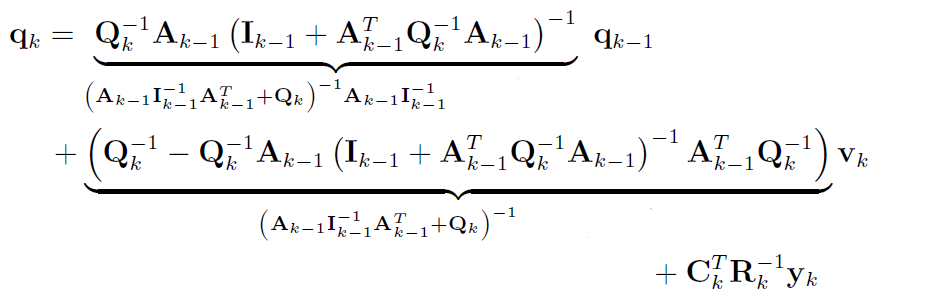
由b式解出 $d_{k-1}$,由c式解出 $L_{k,k-1}$,相乘得到 $L_{k,k-1}d_{k-1}$:

-
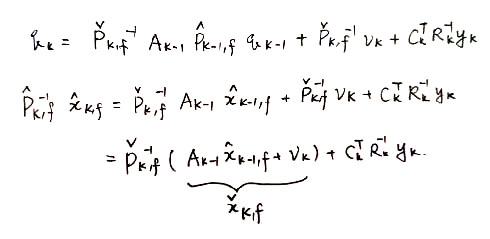
将a式代入上述式子,并将所得式子代入e式,并通过两次SMW变换:
-
用 协方差部分 3的协方差是信息矩阵的逆,以及协方差两个公式,替代上式信息矩阵部分:
-
且令
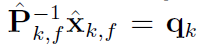
则:
-
整理得到:
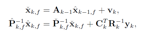
类似于协方差部分 得到了两个式子:
- k的先验均值 由k-1的后验均值预测得出
- k的后验均值 由k的先验均值修正得出 (6进一步用卡尔曼增益变形该式)
-
用卡尔曼增益进一步整理,左右两边同时乘协方差矩阵,右边第一部分根据协方差部分的结论写成(1-KC),第二部分根据K的定义写成K:
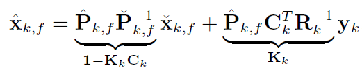

均值更新方程
观察后向迭代式3.66f:
C. 后向迭代
-
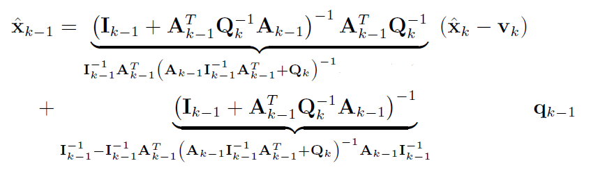
左右同乘 $L_{k-1}$:

-
代入a,b,c式,然后用SMW:
乘进去很快能看出来怎么代入
-
利用之前的公式(A.3, B.4, B.5)代入消去I和q:
写一下很容易代入整理完成

k-1的后验 是 前向后验 + 修正
RTS总结
前向:
1. 先验协方差方程 A.3.1
2. 先验均值方程 B.5.1
3. 卡尔曼增益 A.4
4. 后验协方差更新方程 A.5
5. 后验均值更新方程 B.6
后向:
1. 前向后验修正方程 C.3
使用 前向3 即卡尔曼增益的5个前向式称为
经典形式 canonical form不适用 前向3, 导致 前向4 前向5 用 A.3.2 B.5.2表示的4个式子 称为 逆协方差形式 或
信息形式 information form
SER目录
| SER目录 | ||
|---|---|---|
| SER-1 | K2 - 基础概率论 | |
| SER-2 | K3 - LG系统下Batch/Smoother | |
| SER-3 | K3 - LG系统下Recursive Filter | |
| SER-4 | K4 - NLNG系统下Recursive Filter | |
| SER-5 | K4 - NLNG系统下Batch | |
| SER-6 | K5 - 偏差,匹配和外点 |